【强化学习】8-值函数近似

Categories: RL 2026-03-22

一、例子

到目前为止，我们所看到的状态价值和动作价值都是用表格表示的，以动作价值为例：

	$a_1$	$a_2$	$a_3$	$a_4$	$a_5$
$s_1$	$q_\pi(s_1,a_1)$	$q_\pi(s_1,a_2)$	$q_\pi(s_1,a_3)$	$q_\pi(s_1,a_4)$	$q_\pi(s_1,a_5)$
$\vdots$	$\vdots$	$\vdots$	$\vdots$	$\vdots$	$\vdots$
$s_9$	$q_\pi(s_9,a_1)$	$q_\pi(s_9,a_2)$	$q_\pi(s_9,a_3)$	$q_\pi(s_9,a_4)$	$q_\pi(s_9,a_5)$

优点：直观且易于分析。
缺点：难以处理大规模或连续的状态或动作空间。

考虑一个例子：

假设有一维状态 $s_1, \ldots, s_{|\mathcal{S}|}$，其中 $|\mathcal{S}|=n$ 代表状态空间的状态个数。
它们的状态价值为 $v_\pi(s_1), \ldots, v_\pi(s_{|\mathcal{S}|})$，其中 $\pi$ 是一个给定的策略。
假设 $|\mathcal{S}|$ 非常大，我们希望用一个简单的曲线来逼近这些点，以节省存储空间。

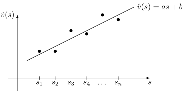
首先，我们使用最简单的直线来拟合这些点。假设直线方程为：

\[\begin{equation} \hat{v}(s, w) = a s + b = \underbrace{[s, 1]}_{\phi^T(s)} \underbrace{\begin{bmatrix} a \\ b \end{bmatrix} }_{w} = \phi^T(s) w \end{equation}\]

其中：

$w$ 是参数向量
$\phi(s)$ 是 $s$ 的特征向量
$\hat{v}(s, w)$ 关于 $w$ 是线性的

优点：

表格表示需要存储 $|\mathcal{S}|$ 个状态价值。而现在，我们只需要存储两个参数 $a$ 和 $b$。
每次我们需要使用状态 $s$ 的价值时，可以通过计算 $\phi^T(s)w$ 来得到。
这种好处并非没有代价：其代价是状态价值无法被精确表示。

其次，我们也可以用二阶曲线来拟合这些点：

\[\begin{equation} \hat{v}(s, w) = a s^2 + b s + c = \underbrace{[s^2, s, 1]}_{\phi^T(s)} \underbrace{\begin{bmatrix} a \\ b \\ c \end{bmatrix} }_{w} = \phi^T(s) w \end{equation}\]

在这种情况下：

$w$ 和 $\phi(s)$ 的维度增加了，但价值可能拟合得更精确。
虽然 $\hat{v}(s, w)$ 关于 $s$ 是非线性的，但关于 $w$ 是线性的。非线性包含在 $\phi(s)$ 中。

我们可以使用更高阶的多项式曲线或其他复杂曲线来拟合这些点：

优点：逼近效果更好。
缺点：需要更多参数。

简要总结一下：

核心思想：使用参数化函数来逼近状态价值和动作价值：$\hat{v}(s, w) \approx v_\pi(s)$，其中 $w \in \mathbb{R}^m$ 是参数向量。
关键区别：访问和赋值 $v(s)$ 的方式不同。
优点：
1. 存储：$w$ 的维度可能远小于 $|\mathcal{S}|$。
2. 泛化：当访问状态 $s$ 时，参数 $w$ 被更新，这样其他一些未访问状态的价值也可以被更新。

二、状态价值估计算法

1. 目标函数

令 $v_\pi(s)$ 和 $\hat{v}(s, w)$ 分别为真实状态价值和用于逼近的函数。我们的目标是找到一个最优的 $w$，使得 $\hat{v}(s, w)$ 能够对每个 $s$ 最好地逼近 $v_\pi(s)$。这实际上是一个策略评估问题，要找到最优的 $w$，我们需要两个步骤：

第一步是定义目标函数。
第二步是推导优化目标函数的算法。

目标函数为：

\[\begin{equation} J(w) = \mathbb{E}\left[(v_\pi(S) - \hat{v}(S, w))^2\right] \end{equation}\]

我们的目标是找到能最小化 $J(w)$ 的最佳 $w$。需要指出的是，这里的期望是关于随机变量 $S \in \mathcal{S}$ 的，那么 $S$ 的概率分布是什么？换句话来说，上式的期望实际上是在做平均，那么怎么进行平均？

第一种方法是使用均匀分布。

即通过将每个状态的概率设为 $1/|\mathcal{S}|$，将所有状态视为同等重要。
在这种情况下，目标函数变为
\[\begin{equation} J(w) = \mathbb{E}[(v_\pi(S) - \hat{v}(S, w))^2] = \frac{1}{|\mathcal{S}|} \sum_{s \in \mathcal{S} } (v_\pi(s) - \hat{v}(s, w))^2 \end{equation}\]

缺点：

状态可能并非同等重要。例如，某些状态可能被策略很少访问到。因此，这种方法没有考虑在给定策略下马尔可夫过程的真实动态特性。

第二种方法是使用平稳分布。

平稳分布描述了马尔可夫过程的长期行为。
令 ${d_\pi(s)}_{s \in \mathcal{S} }$ 表示在策略 $\pi$ 下马尔可夫过程的平稳分布。根据定义，$d_\pi(s) \ge 0$ 且 $\sum_{s \in \mathcal{S} } d_\pi(s) = 1$。
目标函数可以重写为
\[\begin{equation} J(w) = \mathbb{E}[(v_\pi(S) - \hat{v}(S, w))^2] = \sum_{s \in \mathcal{S} } d_\pi(s) (v_\pi(s) - \hat{v}(s, w))^2 \end{equation}\]
这是一个加权平方误差。
由于更频繁访问的状态具有更高的 $d_\pi(s)$ 值，它们在目标函数中的权重也高于那些很少访问的状态。

2. 优化算法

有了目标函数，下一步就是优化它。为了最小化目标函数 $J(w)$，我们可以使用梯度下降算法：

\[\begin{equation} w_{k+1} = w_k - \alpha_k \nabla_w J(w_k) \end{equation}\]

真实的梯度是：

\[\begin{equation} \begin{aligned} \nabla_w J(w) &= \nabla_w \mathbb{E}\left[(v_\pi(S) - \hat{v}(S, w))^2\right] \\ &= \mathbb{E}\left[\nabla_w (v_\pi(S) - \hat{v}(S, w))^2\right] \\ &= 2\mathbb{E}\left[(v_\pi(S) - \hat{v}(S, w))(-\nabla_w \hat{v}(S, w))\right] \\ &= -2\mathbb{E}\left[(v_\pi(S) - \hat{v}(S, w)) \nabla_w \hat{v}(S, w)\right] \end{aligned} \end{equation}\]

上面的真实梯度涉及期望的计算，我们可以使用随机梯度代替真实梯度：

\[\begin{equation} w_{t+1} = w_t + \alpha_t \left(v_\pi(s_t) - \hat{v}(s_t, w_t)\right) \nabla_w \hat{v}(s_t, w_t) \end{equation}\]

其中 $s_t$ 是 $S$ 的一个样本。这里，$2\alpha_k$ 合并成了 $\alpha_k$。

这个算法不可实现，因为它需要真实的状态价值 $v_\pi$，而这正是待估计的未知量。
我们可以用近似值替换 $v_\pi(s_t)$，使得算法可以实现。

具体来说，可以有以下两种方法：

基于 MC 的方法：

令 $g_t$ 为从 $s_t$ 开始的 episode 的折扣回报，那么，$g_t$ 可以用来近似 $v_\pi(s_t)$。算法变为：

\[\begin{equation} w_{t+1} = w_t + \alpha_t (g_t - \hat{v}(s_t, w_t)) \nabla_w \hat{v}(s_t, w_t) \end{equation}\]

基于 TD 的方法：

根据 TD 算法的精髓，$r_{t+1} + \gamma \hat{v}(s_{t+1}, w_t)$ ，即 TD target可以被视为 $v_\pi(s_t)$ 的一个近似。那么，算法变为：

\[\begin{equation} w_{t+1} = w_t + \alpha_t \left[r_{t+1} + \gamma \hat{v}(s_{t+1}, w_t) - \hat{v}(s_t, w_t)\right] \nabla_w \hat{v}(s_t, w_t) \end{equation}\]

3. 伪代码

基于 TD 算法的伪代码如下：

\[\begin{equation*} \begin{aligned} & \text{Initialization: A function } \hat{v}(s, w) \text{ that is differentiable in } w. \text{ Inital parameter } w_0. \\ & \text{Aim: Approximate the true state values of a given policy } \pi \\ & \text{For each episode generated following the policy } \pi, \text{ do} \\ & \quad \quad \text{For each step } (s_t, r_{t+1}, s_{t+1}), \text{ do} \\ & \quad \quad \quad \quad \text{In the general case.} \\ & \quad \quad \quad \quad \quad \quad w_{t+1} = w_t + \alpha_t \left[r_{t+1} + \gamma \hat{v}(s_{t+1}, w_t) - \hat{v}(s_t, w_t)\right] \nabla_w \hat{v}(s_t, w_t) \\ & \quad \quad \quad \quad \text{In the linear case.} \\ & \quad \quad \quad \quad \quad \quad w_{t+1} = w_t + \alpha_t \left[r_{t+1} + \gamma \phi^T(s_{t+1}) w_t - \phi^T(s_t) w_t\right] \phi(s_t) \end{aligned} \end{equation*}\]

该算法只能估计给定策略的状态价值，但对于理解稍后介绍的其他算法很重要。其中，Linear case 是一种特定的 $\hat v$ 的选择，即假设对 $w_t$ 是线性的，后面会介绍。

4. 函数逼近器的选择

一个尚未回答的重要问题：如何选择函数 $\hat{v}(s, w)$？

第一种方法是使用线性函数
\[\begin{equation} \hat{v}(s, w) = \phi^T(s) w \end{equation}\]
这里，$\phi(s)$ 是特征向量，可以是多项式基、傅里叶基等。
第二种方法是使用神经网络作为非线性函数逼近器。神经网络的输入是状态，输出是 $\hat{v}(s, w)$，网络参数是 $w$。

在线性情况下 $\hat{v}(s, w) = \phi^T(s) w$，我们有

\[\begin{equation} \nabla_w \hat{v}(s, w) = \phi(s) \end{equation}\]

将该梯度代入 TD 算法

\[\begin{equation} w_{t+1} = w_t + \alpha_t \left[r_{t+1} + \gamma \hat{v}(s_{t+1}, w_t) - \hat{v}(s_t, w_t)\right] \nabla_w \hat{v}(s_t, w_t) \end{equation}\]

得到

\[\begin{equation} w_{t+1} = w_t + \alpha_t \left[r_{t+1} + \gamma \phi^T(s_{t+1}) w_t - \phi^T(s_t) w_t\right] \phi(s_t) \end{equation}\]

这就是带线性函数逼近的 TD Learning 算法，简称为 TD-Linear。

线性函数逼近的缺点：
- 难以选择合适的特征向量。
线性函数逼近的优点：
- TD 算法在线性情况下的理论性质比非线性情况更容易理解。
- 线性函数逼近仍然强大，因为表格表示是线性函数逼近的一个特例。

我们接下来展示表格表示是线性函数逼近的一个特例：

首先，考虑状态 $s$ 的特殊特征向量：

\[\begin{equation} \phi(s) = e_s \in \mathbb{R}^{|\mathcal{S}|} \end{equation}\]

其中 $e_s$ 是一个第 $s$ 项为 1、其他项为 0 的向量。在这种情况下：

\[\begin{equation} \hat{v}(s, w) = e_s^T w = w(s) \end{equation}\]

其中 $w(s)$ 是 $w$ 的第 $s$ 项。

回顾 TD-Linear 算法是

\[\begin{equation} w_{t+1} = w_t + \alpha_t \left[r_{t+1} + \gamma \phi^T(s_{t+1}) w_t - \phi^T(s_t) w_t\right] \phi(s_t) \end{equation}\]

当 $\phi(s_t) = e_s$ 时，上述算法变为

\[\begin{equation} w_{t+1} = w_t + \alpha_t \left(r_{t+1} + \gamma w_t(s_{t+1}) - w_t(s_t)\right) e_{s_t} \end{equation}\]

这是一个向量方程，只更新 $w_t$ 的第 $s_t$ 项。在等式两边乘以 $e_{s_t}^T$ 得到：

\[\begin{equation} w_{t+1}(s_t) = w_t(s_t) + \alpha_t \left(r_{t+1} + \gamma w_t(s_{t+1}) - w_t(s_t)\right) \end{equation}\]

这正是表格形式的 TD 算法。

三、带 function approximation 的 Sarsa

到目前为止，我们只考虑了状态价值估计的问题。也就是说，我们希望

\[\begin{equation} \hat{v} \approx v_\pi \end{equation}\]

为了寻找最优策略，我们需要估计动作价值。带 function approximation 的 Sarsa 算法为：

\[\begin{equation} w_{t+1} = w_t + \alpha_t \left[r_{t+1} + \gamma \hat{q}(s_{t+1}, a_{t+1}, w_t) - \hat{q}(s_t, a_t, w_t)\right] \nabla_w \hat{q}(s_t, a_t, w_t) \end{equation}\]

这与我们之前介绍的算法相同，只是将 $\hat{v}$ 替换为 $\hat{q}$。为了寻找最优策略，我们可以结合策略评估和策略改进，伪代码如下：

\[\begin{equation*} \begin{aligned} & \text{Aim: Search a good policy that can lead the agent to the target from an initial state-action pair } (s_0, a_0). \\ & \text{For each episode, do} \\ & \quad \quad \text{If the current } s_t \text{ is not the target state, do} \\ & \quad \quad \quad \quad \text{Take action } a_t \text{ following } \pi_t(s_t), \text{ generate } r_{t+1}, s_{t+1}, \text{ and then take action } \\ & \quad \quad \quad \quad a_{t+1} \text{ following } \pi_t(s_{t+1}) \\ & \quad \quad \quad \quad \text{Value update (parameter update):} \\ & \quad \quad \quad \quad \quad \quad w_{t+1} = w_t + \alpha_t \left[r_{t+1} + \gamma \hat{q}(s_{t+1}, a_{t+1}, w_t) - \hat{q}(s_t, a_t, w_t)\right] \nabla_w \hat{q}(s_t, a_t, w_t) \\ & \quad \quad \quad \quad \text{Policy update:} \\ & \quad \quad \quad \quad \quad \quad \pi_{t+1}(a|s_t) = 1 - \frac{\varepsilon}{|\mathcal{A}(s)|}(|\mathcal{A}(s)| - 1) \quad \text{if} \quad a = \arg\max_{a \in \mathcal{A}(s_t)} \hat{q}(s_t, a, w_{t+1}) \\ & \quad \quad \quad \quad \quad \quad \pi_{t+1}(a|s_t) = \frac{\varepsilon}{|\mathcal{A}(s)|} \quad \text{otherwise} \end{aligned} \end{equation*}\]

四、带 function approximation 的 Q-learning

与 Sarsa 类似，表格型 Q-learning 也可以扩展到价值函数逼近的情况，算法为：

\[\begin{equation} w_{t+1} = w_t + \alpha_t \left[r_{t+1} + \gamma \max_{a \in \mathcal{A}(s_{t+1})} \hat{q}(s_{t+1}, a, w_t) - \hat{q}(s_t, a_t, w_t)\right] \nabla_w \hat{q}(s_t, a_t, w_t) \end{equation}\]

这与 Sarsa 相同，只是将 $\hat{q}(s_{t+1}, a_{t+1}, w_t)$ 替换为 $\max_{a \in \mathcal{A}(s_{t+1})} \hat{q}(s_{t+1}, a, w_t)$。

伪代码如下（on-policy 版本）：

\[\begin{equation*} \begin{aligned} & \text{Initialization: Initial parameter vector } w_0. \text{ Initial policy } \pi_0. \text{ Small } \varepsilon > 0. \\ & \text{Aim: Search a good policy that can lead the agent to the target from an initial state-action pair } (s_0, a_0). \\ & \text{For each episode, do} \\ & \quad \quad \text{If the current } s_t \text{ is not the target state, do} \\ & \quad \quad \quad \quad \text{Take action } a_t \text{ following } \pi_t(s_t), \text{ generate } r_{t+1}, s_{t+1} \\ & \quad \quad \quad \quad \text{Value update (parameter update):} \\ & \quad \quad \quad \quad \quad \quad w_{t+1} = w_t + \alpha_t \left[r_{t+1} + \gamma \max_{a \in \mathcal{A}(s_{t+1})} \hat{q}(s_{t+1}, a, w_t) - \hat{q}(s_t, a_t, w_t)\right] \nabla_w \hat{q}(s_t, a_t, w_t) \\ & \quad \quad \quad \quad \text{Policy update:} \\ & \quad \quad \quad \quad \quad \quad \pi_{t+1}(a|s_t) = 1 - \frac{\varepsilon}{|\mathcal{A}(s)|}(|\mathcal{A}(s)| - 1) \quad \text{if} \quad a = \arg\max_{a \in \mathcal{A}(s_t)} \hat{q}(s_t, a, w_{t+1}) \\ & \quad \quad \quad \quad \quad \quad \pi_{t+1}(a|s_t) = \frac{\varepsilon}{|\mathcal{A}(s)|} \quad \text{otherwise} \end{aligned} \end{equation*}\]

五、Deep Q-learning

Deep Q-learning 是最早、最成功的将深度神经网络引入强化学习的算法之一。神经网络的作用是作为一个非线性函数逼近器。与以下的 Q-learning 的算法不同：

Deep Q-learning 由于引入神经网络，不再使用这么底层的方法。Deep Q-learning 旨在最小化目标函数/损失函数：

\[\begin{equation} J(w) = \mathbb{E}\left[\left(R + \gamma \max_{a \in \mathcal{A}(S')} \hat{q}(S', a, w) - \hat{q}(S, A, w)\right)^2\right] \label{eq:obj} \end{equation}\]

其中 $(S, A, R, S’)$ 是随机变量。这实际上是贝尔曼最优误差。这是因为：

\[\begin{equation} q(s, a) = \mathbb{E}\left[R_{t+1} + \gamma \max_{a \in \mathcal{A}(S_{t+1})} q(S_{t+1}, a) \mid S_t = s, A_t = a\right], \quad \forall s, a \end{equation}\]

在期望意义上，$R + \gamma \max_{a \in \mathcal{A}(S’)} \hat{q}(S’, a, w) - \hat{q}(S, A, w)$ 的值应该为零。

我们使用梯度下降方法来最小化该目标函数，在目标函数 $\eqref{eq:obj}$ 中，参数 $w$ 不仅出现在 $\hat{q}(S, A, w)$ 中，也出现在

\[\begin{equation} y \doteq R + \gamma \max_{a \in \mathcal{A}(S')} \hat{q}(S', a, w) \end{equation}\]

为了简化，我们可以假设在计算梯度时，$y$ 中的 $w$ 是固定的（至少在一段时间内）。

为此，我们可以引入两个网络。

一个是主网络 (main network)，表示 $\hat{q}(s, a, w)$。
另一个是目标网络 (target network)，$\hat{q}(s, a, w_T)$。

在这种情况下，目标函数简化为：

\[\begin{equation} J = \mathbb{E}\left[\left(R + \gamma \max_{a \in \mathcal{A}(S')} \hat{q}(S', a, w_T) - \hat{q}(S, A, w)\right)^2\right] \end{equation}\]

其中 $w_T$ 是目标网络参数。当 $w_T$ 固定时，$J$ 的梯度可以容易地求得为（这里省略系数 2）：

\[\begin{equation} \nabla_w J = \mathbb{E}\left[\left(R + \gamma \max_{a \in \mathcal{A}(S')} \hat{q}(S', a, w_T) - \hat{q}(S, A, w)\right) \nabla_w \hat{q}(S, A, w)\right] \end{equation}\]

这一优化过程涉及到两个技巧。第一个技巧即引入两个网络，它的实现细节如下：

令 $w$ 和 $w_T$ 分别表示主网络和目标网络的参数。它们初始时设置为相同。
在每次迭代中，我们从经验回放缓冲区 (replay buffer)中抽取一小批样本 ${(s, a, r, s’)}$。
网络的输入包括状态 $s$ 和动作 $a$。目标输出是 $y_T \doteq r + \gamma \max_{a \in \mathcal{A}(s’)} \hat{q}(s’, a, w_T)$。然后，我们直接在小批量 ${(s, a, y_T)}$ 上最小化 TD error （即损失函数 $(y_T - \hat{q}(s, a, w))^2$）。

第二个技巧是经验回放 (Experience Replay)。在我们收集了一些经验样本后，我们不会按照收集的顺序使用这些样本。相反，我们将它们存储在一个集合中，称为回放缓冲区 (replay buffer) $\mathcal{B} \doteq {(s, a, r, s’)}$。每次我们训练神经网络时，我们可以从回放缓冲区中随机抽取一小批样本。样本的抽取，称为经验回放，它应该遵循均匀分布。在目标函数中：

\[\begin{equation} J = \mathbb{E}\left[\left(R + \gamma \max_{a \in \mathcal{A}(S')} \hat{q}(S', a, w) - \hat{q}(S, A, w)\right)^2\right] \end{equation}\]

$(S, A) \sim d$：$(S, A)$ 作为一个索引，被视为一个单一的随机变量（理解为二维平面上一个点的坐标）。
$R \sim p(R|S, A), S’ \sim p(S’|S, A)$：$R$ 和 $S’$ 由系统模型决定。
状态-动作对 $(S, A)$ 的分布被假设为均匀分布。
然而，样本并不是均匀收集的，因为它们是由特定策略依次生成的。
为了打破连续样本之间的相关性，我们可以使用经验回放技术，从回放缓冲区中均匀抽取样本。
这就是为什么经验回放是必要的，以及为什么经验回放必须是均匀分布的数学原因。

Deep Q-learning 的伪代码如下（off-policy 版本）：

\[\begin{equation*} \begin{aligned} & \text{Aim: Learn an optimal target network to approximate the optimal action values from the experience} \\ & \text{samples generated by a behavior policy } \pi_b. \\ & \text{Store the experience samples generated by } \pi_b \text{ in a replay buffer } \mathcal{B} = \{(s, a, r, s')\} \\ & \quad \quad \text{For each iteration, do} \\ & \quad \quad \quad \quad \text{Uniformly draw a mini-batch of samples from } \mathcal{B} \\ & \quad \quad \quad \quad \text{For each sample } (s,a,r,s'), \text{ calculate the target value as } y_T = r + \gamma \max_{a \in \mathcal{A}(s')} \hat{q}(s', a, w_T), \\ & \quad \quad \quad \quad \text{where } w_T \text{ is the parameter of the target network.} \\ & \quad \quad \quad \quad \text{Update the main network to minimize } (y_T - \hat{q}(s, a, w))^2 \text{ using the mini-batch } \{(s,a,y_T)\} \\ & \quad \quad \text{Set } w_T = w \text{ every } C \text{ iterations.} \\ \end{aligned} \end{equation*}\]

参考

强化学习的数学原理